COVID-19: Aerosol and Surface Stability of SARS-CoV-2

Viruses didn’t become ubiquitous by being wimps: From the rhinoviruses that cause the common cold to the new coronavirus that has spread across the world, they are able to survive on surfaces far away from the living cells that they need in order to reproduce. How long they can lurk before a living organism comes along to infect depends on the kind of surface and the properties of the virus: The Covid-19 virus, according to a new study, sticks around on plastic surfaces for up to three days, but for a shorter period on metals.

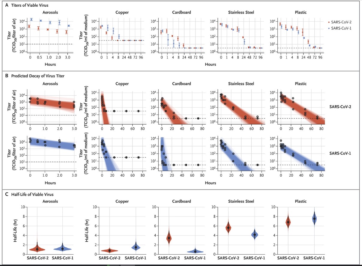
The survival of the coronavirus on surfaces is similar to that of the SARS virus, to which it’s related. On plastic, after eight hours only 10% of what researchers deposited was still there, according to a study published on Tuesday in the New England Journal of Medicine. But the virus didn’t become undetectable until after 72 hours. On stainless steel, the numbers began plummeting after just four hours, becoming undetectable by about 48 hours. On copper and cardboard, virus was undetectable by eight hours and 48 hours, respectively.

The fewer the virus particles on a surface, the lower the chances that someone touching it will become infected. “You have to get a certain level of virus exposure to be infected,” said Ross McKinney, chief scientific officer of the American Association of Medical Colleges. And infection cannot happen through the skin: to “self inoculate,” one must transfer virus from, say, the fingers to the nose or eyes, where it can enter the body via mucus membranes.

Source: statnews.com/